Categories
Climbing

Climbing at Index (April 26th)

Leaving Seattle at 7:30, I got to Index and met up with Cameron a little after 9. Then we headed over to our first climb of the day. It was the “ss-ultrabrutal”. I am glad I found about the name after we climbed it – that name is just awesomely intimidating.

It is a trad climb, Cameron led and I cleaned. At the time I thought it was just a 5.6 (it’s a 5.7) but it was an easy climb, and I had hard time on it, so while I enjoyed myself I came off it just feeling a little depressed about how out of climbing shape I was. Definitely time to hit the gym more. In the picture you can just make out Cameron at the bolts at the top of the climb. The climb traverses left to right on about a forty five degree angle – following the large crack above the old tunnel.

IMG_0023b

Next we moved over to do the GM route on The Country. Cameron had climbed it before and wanted to lead all three pitches in a single push. So I belayed him from the ground, then he rappelled back down to the first pitch belay ledge cleaning as he went. I’d thought I’d be doing the second two pitches, but I just made such a mess of cleaning the first pitch Cameron just pulled the rope and I cleaned the first pitch. You can see the rope line in the picture. Cameron had already been doing some rope soloing that morning – and I was having an off day – so we called it and went and put our heads in the river.

IMG_0025

Think I am kidding? Nope. Cameron put his head in the river and it looked so refreshing I followed suit.

IMG_0039

All in all a lovely day – but I confess after seeing the camping spot he snagged by showing up on a Wednesday, I was kicking myself for not joining the night before. I skipped the over night so I could attend a practice session on glacier travel. Lesson learned.

IMG_0035

The view from the river was even better.

IMG_0037

Categories
Programming

NetworkX Graph library for Python

I’ll admit – I still try and write Python like it was C or C++. To fix that for a while I am going to switch to writing things in Python for a while, while working on actually writing good Python.

Graph algorithms are the kidneys of computer science – there in the background filtering out all the bad things for us. In my switch over to writing in Python I needed to find a solid python graph library, and decided to try NetworkX. Here is a simple example program using it. These are mostly just notes for myself – but I am posting it here in case it is useful to anyone else.

This code is basically the NetworkX weighted graph example, with some annotations. Here is some code to create and plot a weighted graph.


import matplotlib.pyplot as plt
import networkx as nx

# Populate the graph...
map_graph = nx.Graph()

map_graph.add_edge('Issaquah','Bellevue', weight=0.11 )
map_graph.add_edge('Bellevue','Kirkland', weight=0.05 )
map_graph.add_edge('Bellevue','Redmond', weight=0.06 )
map_graph.add_edge('Kirkland','Redmond', weight=0.24 )
map_graph.add_edge('Bellevue','Seattle', weight=0.01 )
map_graph.add_edge('Renton','Seattle', weight=0.03 )
map_graph.add_edge('Renton','Bellevue', weight=0.48 )

# Determine the layout of points in the graph. Some other layouts that 
# would work here are spring_layout, shell_layout, and random_layout                                                                                                 
pos = nx.circular_layout( map_graph ) # Sets positions for nodes

# Put "dots" down for each node                                                     
nx.draw_networkx_nodes( map_graph, pos, node_size=700)

# Attaches Labesl to each node                                                               
nx.draw_networkx_labels( map_graph, pos, font_size=14, font_family='sans-serif')

map_edges = [(u,v) for (u, v, d) in map_graph.edges(data=True) ]

nx.draw_networkx_edges( map_graph,
                        pos,             # Spring
                        map_edges,       # List of edges                                     
                        width=5, alpha=0.5, edge_color='b', style='dashed' )

plt.axis('off')
plt.show()

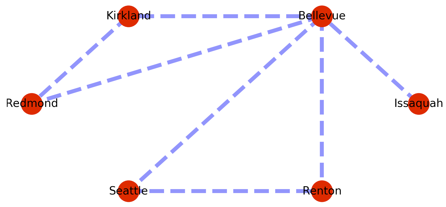
The plotted graph looks something like this.

Screen Shot 2018-04-29 at 5.01.30 PM

One of the things I want from a graph library is the standard graph algorithms – like finding me the shortest path between nodes, or testing for the presence of a path at all. So for example to find the shortest path from Issaquah to Renton we could add the following code to the example above?:


# Generates the shortest path - but since there could be more than                                                   
# one of them what you get back is a "generator" from which you                                                      
# need to pluck the shortest path.                                                                                   
a_shortest_path = nx.all_shortest_paths(map_graph, source='Issaquah', target='Renton')                              

print( [p for p in a_shortest_path] )    

The added code will give the path [[‘Issaquah’, ‘Bellevue’, ‘Renton’]], which is the shortest path by number of edges traversed. To obtain the shortest path by edge weight we can use dijkstras like so:


a_shortest_path = nx.dijkstra_path(map_graph, ‘Issaquah’, ‘Renton’)
print( a_shortest_path )

Which gives the path: [‘Issaquah’, ‘Bellevue’, ‘Seattle’, ‘Renton’]

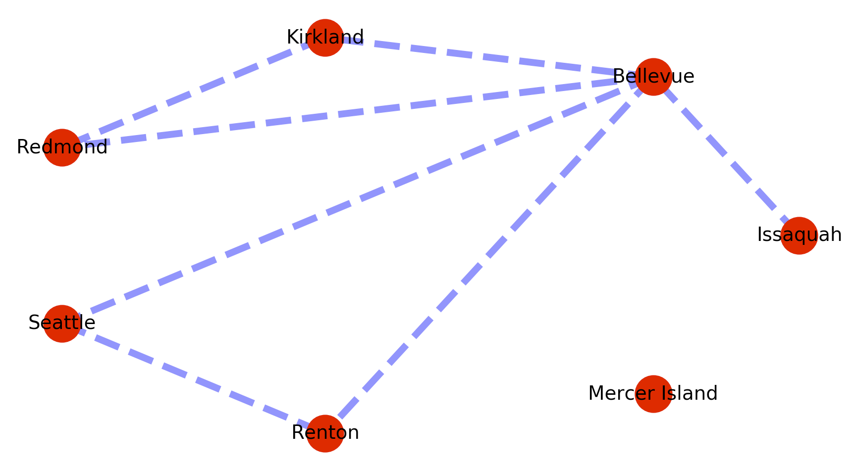
The problem is that this implementation of dijkstra’s fails when a path is not present between the origin and destination nodes. So for example if we add a disconnected vertex with no edges like below, searches on a path to that vertex will cause the call to fail.


map_graph.add_node(‘Mercer Island’)

Screen Shot 2018-04-29 at 8.15.15 PM

I think you need to use the has_path method to test for the existence of any path first, then if there is a path use dijkstras to find the minimum cost path. Something like this:


# Create a helper function for testing for a path
def shortest_weighted(from_node, to_node):
    if nx.has_path( map_graph, from_node, to_node ) == True :
	a_shortest_path = nx.dijkstra_path(map_graph, from_node, to_node)
        return( a_shortest_path )
    else:
        print("No path from",from_node,"to", to_node, "\r\n")
        return( False )

Then checking for the minimum path can look something like this:


# Test where path does not exist
shortest_weighted_path = shortest_weighted( 'Issaquah', 'Mercer Island' )
if shortest_weighted_path != False:
    print( shortest_weighted_path )

# Test where path does exist
shortest_weighted_path = shortest_weighted( 'Issaquah', 'Renton' )
if shortest_weighted_path != False:
    print( shortest_weighted_path )

Neither call will fail and checking for the existing path from Issaquah to Renton will return: [‘Issaquah’, ‘Bellevue’, ‘Seattle’, ‘Renton’]

Since the graphs are weighted – list comprehensions can be used to conditionally act based on edge weights. For example:


# Segment the nodes by weight                                                                                                  
map_red_edges  = [(u,v) for (u, v, d) in map_graph.edges(data=True) if d['weight'] >  0.1  ]
map_blue_edges = [(u,v) for (u, v, d) in map_graph.edges(data=True) if d['weight'] <= 0.1  ]

Then use the segmentation to perform multiple colorings.


nx.draw_networkx_edges( map_graph,
                        pos,             # Spring                                                                    
                        map_red_edges,   # List of edges                                                             
                        width=5,
                        alpha=0.5,
                        edge_color='r',
                        style='dashed' )

nx.draw_networkx_edges( map_graph,
                        pos,             # Spring                                                                    
                        map_blue_edges,  # List of edges                                                             
                        width=5,
                        alpha=0.5,
                        edge_color='b',
                        style='solid' )

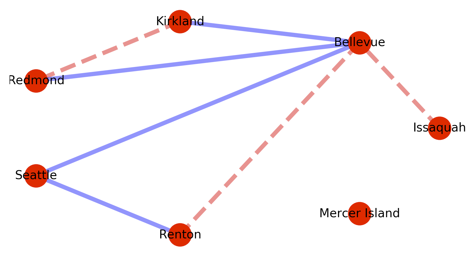
Which will produce the following graph:

Screen Shot 2018-04-29 at 9.49.43 PM

Also useful is shortest_path, which returns all the paths between all nodes, but sorted by vertex traversal path length. So the following code:


paths = nx.shortest_path(map_graph)
print( paths )

Generates the following paths.


{'Issaquah': {'Issaquah': ['Issaquah'], 'Bellevue': ['Issaquah', 'Bellevue'], 'Kirkland': ['Issaquah', 'Bellevue', 'Kirkland'], 'Redmond': ['Issaquah', 'Bellevue', 'Redmond'], 'Seattle': ['Issaquah', 'Bellevue', 'Seattle'], 'Renton': ['Issaquah', 'Bellevue', 'Renton']}, 'Bellevue': {'Bellevue': ['Bellevue'], 'Issaquah': ['Bellevue', 'Issaquah'], 'Kirkland': ['Bellevue', 'Kirkland'], 'Redmond': ['Bellevue', 'Redmond'], 'Seattle': ['Bellevue', 'Seattle'], 'Renton': ['Bellevue', 'Renton']}, 'Kirkland': {'Kirkland': ['Kirkland'], 'Bellevue': ['Kirkland', 'Bellevue'], 'Redmond': ['Kirkland', 'Redmond'], 'Issaquah': ['Kirkland', 'Bellevue', 'Issaquah'], 'Seattle': ['Kirkland', 'Bellevue', 'Seattle'], 'Renton': ['Kirkland', 'Bellevue', 'Renton']}, 'Redmond': {'Redmond': ['Redmond'], 'Bellevue': ['Redmond', 'Bellevue'], 'Kirkland': ['Redmond', 'Kirkland'], 'Issaquah': ['Redmond', 'Bellevue', 'Issaquah'], 'Seattle': ['Redmond', 'Bellevue', 'Seattle'], 'Renton': ['Redmond', 'Bellevue', 'Renton']}, 'Seattle': {'Seattle': ['Seattle'], 'Bellevue': ['Seattle', 'Bellevue'], 'Renton': ['Seattle', 'Renton'], 'Issaquah': ['Seattle', 'Bellevue', 'Issaquah'], 'Kirkland': ['Seattle', 'Bellevue', 'Kirkland'], 'Redmond': ['Seattle', 'Bellevue', 'Redmond']}, 'Renton': {'Renton': ['Renton'], 'Seattle': ['Renton', 'Seattle'], 'Bellevue': ['Renton', 'Bellevue'], 'Issaquah': ['Renton', 'Bellevue', 'Issaquah'], 'Kirkland': ['Renton', 'Bellevue', 'Kirkland'], 'Redmond': ['Renton', 'Bellevue', 'Redmond']}, 'Mercer Island': {'Mercer Island': ['Mercer Island']}}

Categories
Down wind of the future Machine Learning

DeepFakes and Jordan Peele’s Obama PSA

This is an awesome PSA about information hygene and the problems that our society is about to face. Basically, breakthroughs in the last few years have been accelerating what you can do with machine learning at a break-neck pace. Since people can kind of suck, not all of that advancement has been for the benefit of society at large.

In late 2017 some equally brilliant and creepy work was released letting someone (super creepy) place the face of anyone for whom they could get a few hundred pictures on a porn star’s body. Basically this was the creation of a new, modern, sex crime. No one wanted to talk about this threat, because – porn. Well, thankfully Jordan Peele and some others put out a PSA about this coming threat. As you can see in this video they have generated video of “President Obama”, saying all sorts of things. The video effectively nailed generation of voice, tone, intonation, gesture, and lighting. Its an awesome fake.

Right know, with a little knowledge about how the video was generated, it is fairly easy to prove its is not authentic. That illustrates the problem though, you quickly start needing to use math to prove that the video is faked. Math is also quickly becoming inherently distrusted by more and more people. We are also not that far from this tech being able to be run reliably in real time. So – generation of a video of any public figure believably saying anything you want them to is not that far off.

The obvious threat is anyone caught committing an undesirable act will soon be able to more believably cry “fake news”. Thats the simpler problem though. The real problem will kick off as soon as people start generating revisionist historical records. That thread – when pulled – could unravel our cultural anchor to the past, changing our understanding of our cultural and societal path to now.

Categories
Machine Learning

Data sets for Machine Learning

Grad school was a few years ago, and things are moving fast, so I am writing a bunch of small ML programs to get current with the state of the art again. Also switching form using C++ to Python for ML work. Wow, thats a huge improvement right there – can’t believe I waited this long.

The biggest problem in writing ML code is finding decent data sets. The UCI Machine Learning Repository has links to a bunch of curated data sets. Posting it here, like the rest of the ML stuff I’m about to, so its easy to find and point friends to.

Categories
Data Machine Learning

Decision Tree Classifiers – A simple example

Here is a simple “Machine Learning” Python program using scikit-learn’s DecisionTree classifier to use height and weight to predict your body type. For the record – this is why people hate BMI and things like it. After writing this I think I need to go on a diet.

Identification Trees – often called decision trees – provide a way to deterministically map a bunch of qualitative observations into predictions. Basically the predictions are a set of observed output states, and we are looking for observable features, inputs, that we can use in a tree of tests.

Training builds the decision tree from two sets of data, our set of observations and a set of labels corresponding to each of the observations. Each node in the tree represents a test that cuts the training set with a number of cuts – the results of each of those cuts going on to either subsequent tests, or to a leaf node representing a specific output label or state.

The MIT open courseware video Identification Trees and Disorder is a good introduction.

So lets say we wanted to determine based on someone’s height and weight if they were overweight or not. To get some training data we could take bunch of random samples of a representative population of people – ask them their height and weight and then create labels for each person determining if they were of a normal weight, overweight, or obese. That would not be a fun data set to try and collect – so lets cheat.

The Body Mass Index or BMI is an equation already derived from population health data that roughly maps height and weight into a number, the BMI. The BMI can be used to predict if a person is under weight, normal weight, and over weight, or obese. The BMI equation is roughly BMI = [(weight in pounds * 703)/(height in inches squared)]. A BMI of less than 18.5 are underweight, BMIs between 19 and 25 reflect a normal weight, a BMI of 25-30 correspond to being overweight, and a BMI over 30 signals obesity. So BMI equations let us build a table mapping height and weight to a table that would be representative of uniform sampling of a large population.

So using BMI sampling data here is a simple Python program using sklearn’s DecisionTree classifier to tell you if you are obese, overweight, or normal weight.


from sklearn import tree

BMI_features = [ “NOR”, “NOR”, … lots of data here … , “OBE”, “OBE”]
Height_in_Weight_lbs_samples = [[91,58],[96,58], … lots of data here … ,[279,76],[287,76]]

# Create identification tree from BMI table.
clf = tree.DecisionTreeClassifier()
clf = clf.fit(Height_in_Weight_lbs_samples, BMI_features)

looping = True
while( looping ):
weight = input(“Enter your weight in lbs: “)
if not weight:
break

height = input(“Enter your height in inches: “)
if not height:
break

prediction = clf.predict([[weight,height]])
print(“It appears that you are:”, prediction, “\r\n” )

Output of the program looks something like this. Yeah, I’m regretting both dessert and choosing this example.


Enter your weight in lbs: 225
Enter your height in inches: 70
It appears that you are: [‘OBE’]

Enter your weight in lbs: 175
Enter your height in inches: 70
It appears that you are: [‘OVE’]

Enter your weight in lbs: 168
Enter your height in inches: 70
It appears that you are: [‘NOR’]

Enter your weight in lbs:

Sometimes it can be useful to look directly at the generated decision tree. This code generates a visualization of the tree.


# Generate a graph visualizing the trained decesion tree.
import graphviz
dot_data = tree.export_graphviz(clf, out_file=None)
graph = graphviz.Source(dot_data)
graph.render(“BMI_Table”, view=True)

I put this code, including the full data sets for training up at: git@github.com:aarontoney/Machine_Learning_Examples.git